Adjusted R-squared for MLR

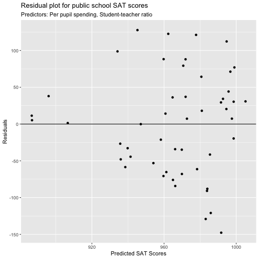
class: center, middle, inverse, title-slide

# Adjusted R-squared for MLR
### STAT 021 with Prof Suzy
### Swarthmore College

---

.scroll-output {
  height: 70%;
  overflow-y: scroll;
}

.scroll-small {
  height: 50%;
  overflow-y: scroll;
}
   
.red{color: #ce151e;}
.green{color: #26b421;}
.blue{color: #426EF0;}
</style>

## The effect of adding more predictor variables in a MLR  
### SAT model with .blue[two] predictors

.scroll-output[

```r
MLR_SAT2 <- lm(SAT_tot ~ PerPupilSpending + 
                         StuTeachRatio, data = SAT_data)
MLR_SAT2_sum <- summary(MLR_SAT2)
MLR_SAT2_sum
```

```
## 
## Call:
## lm(formula = SAT_tot ~ PerPupilSpending + StuTeachRatio, data = SAT_data)
## 
## Residuals:
##      Min       1Q   Median       3Q      Max 
## -147.694  -51.816    6.258   37.756  127.742 
## 
## Coefficients:
##                  Estimate Std. Error t value Pr(>|t|)    
## (Intercept)      1136.336    107.803  10.541 5.69e-14 ***
## PerPupilSpending  -22.308      7.956  -2.804  0.00731 ** 
## StuTeachRatio      -2.295      4.784  -0.480  0.63370    
## ---
## Signif. codes:  0 '***' 0.001 '**' 0.01 '*' 0.05 '.' 0.1 ' ' 1
## 
## Residual standard error: 70.48 on 47 degrees of freedom
## Multiple R-squared:  0.149,	Adjusted R-squared:  0.1128 
## F-statistic: 4.114 on 2 and 47 DF,  p-value: 0.02258
```
]
---
## SAT model with .blue[two] predictors

```r
residual_plot_data2 <- SAT_data %>% 
                      mutate(residuals = MLR_SAT2_sum$residuals,fitted_vals = MLR_SAT2$fitted.values) %>%
                      select(-c(State, SAT_verbal, SAT_math))

ggplot(residual_plot_data2) +
  geom_point(aes(x=fitted_vals, y=residuals)) + 
  labs(title="Residual plot", subtitle="Public school SAT scores", x="Predicted SAT Scores", y="Residuals") + 
  geom_hline(yintercept=0)
```
---
## SAT model with .blue[two] predictors

![](Figs/class20_model2-1.png)

---
## SAT model with .blue[three] predictors
.scroll-output[

```
## 
## Call:
## lm(formula = SAT_tot ~ PerPupilSpending + StuTeachRatio + Salary, 
##     data = SAT_data)
## 
## Residuals:
##      Min       1Q   Median       3Q      Max 
## -140.911  -46.740   -7.535   47.966  123.329 
## 
## Coefficients:
##                  Estimate Std. Error t value Pr(>|t|)    
## (Intercept)      1069.234    110.925   9.639 1.29e-12 ***
## PerPupilSpending   16.469     22.050   0.747   0.4589    
## StuTeachRatio       6.330      6.542   0.968   0.3383    
## Salary             -8.823      4.697  -1.878   0.0667 .  
## ---
## Signif. codes:  0 '***' 0.001 '**' 0.01 '*' 0.05 '.' 0.1 ' ' 1
## 
## Residual standard error: 68.65 on 46 degrees of freedom
## Multiple R-squared:  0.2096,	Adjusted R-squared:  0.1581 
## F-statistic: 4.066 on 3 and 46 DF,  p-value: 0.01209
```
]
---
## SAT model with .blue[three] predictors

---
## SAT model with .blue[three] predictors
### What did we notice?

- As we increase the number of predictor variables, the R-squared value increases;

- Our estimate for `$\sigma$` decreases;

- The shape of the residuals plot changes;

- The significance of any given predictor variable can change;

- The overall F test changes as well.

**Q:** Did anything stay the same?

--
**A:** Not really. Either model choice here is different, which means that these models are what statisticians call *non-robust*.

---
## SAT model with .blue[four] predictors

.scroll-output[

```
## 
## Call:
## lm(formula = SAT_tot ~ PerPupilSpending + StuTeachRatio + Salary + 
##     prop_taking_SAT, data = SAT_data)
## 
## Residuals:
##     Min      1Q  Median      3Q     Max 
## -90.531 -20.855  -1.746  15.979  66.571 
## 
## Coefficients:
##                  Estimate Std. Error t value Pr(>|t|)    
## (Intercept)      1045.972     52.870  19.784  < 2e-16 ***
## PerPupilSpending    4.463     10.547   0.423    0.674    
## StuTeachRatio      -3.624      3.215  -1.127    0.266    
## Salary              1.638      2.387   0.686    0.496    
## prop_taking_SAT  -290.448     23.126 -12.559 2.61e-16 ***
## ---
## Signif. codes:  0 '***' 0.001 '**' 0.01 '*' 0.05 '.' 0.1 ' ' 1
## 
## Residual standard error: 32.7 on 45 degrees of freedom
## Multiple R-squared:  0.8246,	Adjusted R-squared:  0.809 
## F-statistic: 52.88 on 4 and 45 DF,  p-value: < 2.2e-16
```
]
---
## SAT model with .blue[four] predictors

---
## SAT model with .blue[four] predictors
### What did we notice?

Again we see the same patterns as before. But note that our interpretation of the individual effects of each variable changes as well!

---
##R squared
### Why does adding predictor variables increase `$R^2$`?

`$$R^2 = \frac{SS_{reg}}{SS_{tot}} = 1 - \frac{SS_{res}}{SS_{tot}}$$`

What is `$SS_{res}$`?

--
Recall `$Var(\epsilon) = \sigma^2$` and `$\hat{\sigma}^2 = \frac{SS_{res}}{n-2}.$`

The way we determine the coefficients of our linear model (i.e. the `$\hat{\beta}$`'s) is by minimizing `$SS_{res}$`. Mathematically, minimizing `$SS_{res}$` is equivalent to maximizing `$R^2$`.

So this question can be rephrased as: .red[why does adding more predictor variables decrease] `$SS_{res}$`?

---
##R squared
### Why does adding more predictor variables decrease `$SS_{res}$`?

Because we define the regression estimates as the "least squares" estimates. That is, by definition, (in SLR for example)

`$$\hat{\beta_0} = \bar{y} + \hat{\beta_1} \bar{x} \\
\hat{\beta_1} = \frac{\sum_{i=1}^{n}(x_i - \bar{x})(y_i - \bar{y})}{\sum_{i=1}^{n}(x_i - \bar{x})^2}$$`

are the values that minimize `$SS_{res}$`, the squared distance between the data and the line. So as we have to estimate more and more `$\hat{\beta}$`'s, we continue to minimize `$SS_{res}$`, but we are able to make `$SS_{res}$` even smaller than before. The main reason why is the logical fact stated below.

--
  > If set `$S$` has `$n$` elements in it, we can find the minimum and the maximum of this set. If we add `$t>0$` more elements to the set, it is possible that both the minimum and maximum values are more extreme than they were before.

---
## R squared
### R - the programming language - output

In the linear regression output of R we have

- multiple R squared is the R squared that we define as `$R^2 = \frac{SS_{reg}}{SS_{tot}}$`; 
  
- adjusted R squared this imposes a penalty on the multiple R squared value that accounts for adding more predictor variables to the model.